Chapter 8 Additional Modeling techniques.
In this chapter, we will see some additional machine learning models used in practice, for various purpose.
After studying both classification models and regression models in the previous 2 chapters 6 & 7 respectively, we will now look into other generic models used for classification and/or regression purpose.
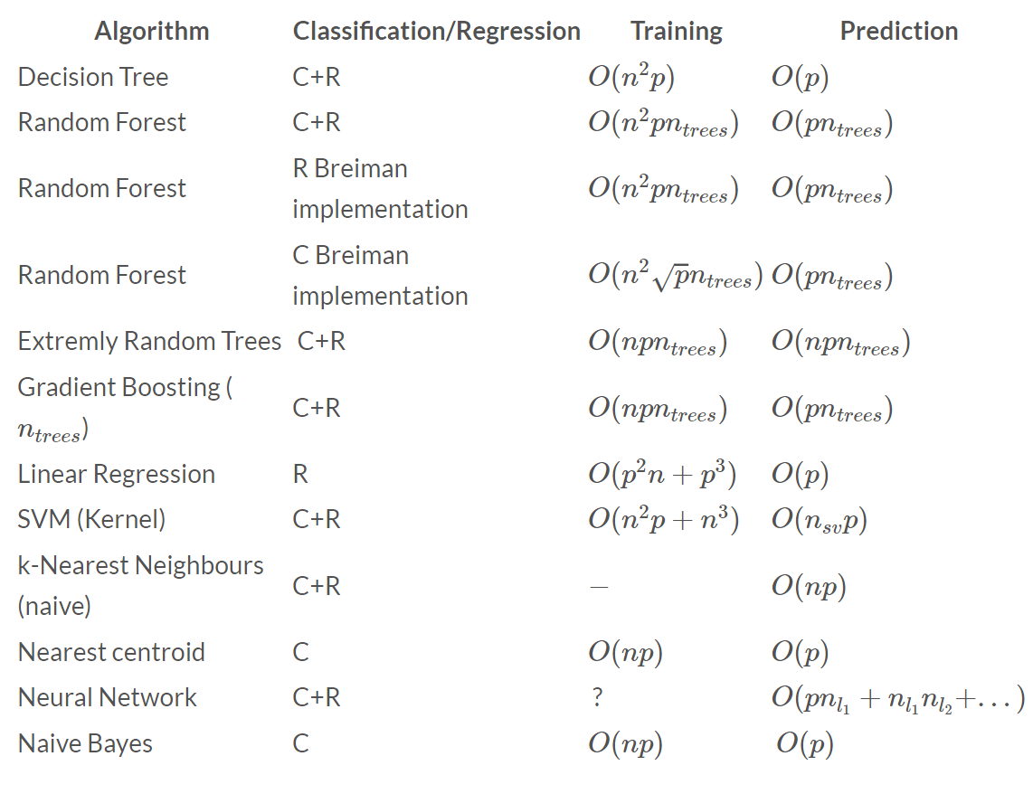
Below is the list some of the widely used algorithms with their use case(either classification/regression or both) and training and prediction complexities for using particular learning models.

Usage and Complexity of various machine learning algorithms. Credits:thekerneltrip.com
As we can see that many of these algorithms can be used for classification and regression all together, as we saw in the case of the Decision tree models using Rpart in section 6.1, and also some model used for only a particular type of prediction e.g. linear regression.
We will look at few algorithms from the above list:
- Random Forest
- Support Vector Machine (SVM)
- Neural Networks
8.1 Four Line Method for creating most type of prediction models in R
But before we learn about these algorithms, let us see a four line method to build models using any of the above algorithms using R.
We can safely assume that the data going to be used to build the model, has been pre-processed and based on requirements split into the required subsets. To see how to split the data refer to section 6.6.
- The zeroth step now will be obviously to install and load the packages that contain the ML algorithm. To do that on your local machine, use the following code.
# Install the library
install.packages("package name")

# Load the library in R
library(package_name)- Once we have the algorithm library loaded, we then proceed to build the model.
pred.model = model_function(formula, data, method*,...)- model_function(): the function present in the library to build the model. e.g. rpart()
- formula: here we mention the prediction column and the other related columns(predictors) on which the prediction will be based on.
prediction ~ predictor1 + predictor2 + predictor3 + ...
- data: here we provide the dataset on which the ML model is to be trained on. Remember never used the test data to build the model.
- method: (OPTIONAL) Used to denote the method of prediction or underlying algorithm. This parameter could be present in some model_function() but not all.
- Prediction using the predict() function on the training data to assess the models performance/accuracy in next step.
pred = predict(pred.model, newdata = train)- predict(): the common function for all models used for prediction.
- pred.model: output of the step 1.
- newdata: here we assign the data on which the prediction is to be done.
- Evaluate error in Training phase. We use the mse() function for finding the accuracy of the model. To read more in dept about the mse() function refer to section 7.1.2.
mse(actual, pred)- actual: vector of the actual values of the attribute we want to predict.
- pred: vector of the predicted values obtained using our model.
Repeat steps 0,1,2 and 3 by changing the ML algorithm or manipulating dataset to perform better when used to train using ML model, so as to achieve as low MSE value as possible.
- Finally we predict on the testing data using the same predict function as in step 2 but replacing the train data with test data.
pred = predict(pred.model, newdata = test)
These are the 4 steps to follow while performing any prediction task using ML models in R.
We can also add one more step between step 3 and 4, which is step of performing the cross validation process on the newly built models.
This can be done either manually, or by using third party libraries.
One such library is the rModeling package, which has function crossValidation() which can be used for any type of model_functions(). For more information visit crossValidation()
Before we proceed to the next section, please look at the snippet of the earnings.csv dataset, which we will be using for predicting the Earnings attribute based on various other attributes provided in the dataset, using different prediction models.
| GPA | Number_Of_Professional_Connections | Earnings | Major | Graduation_Year | Height | Number_Of_Credits | Number_Of_Parking_Tickets | |
|---|---|---|---|---|---|---|---|---|
| 2221 | 2.72 | 36 | 10282.54 | Humanities | 1963 | 69.51 | 122 | 3 |
| 5198 | 1.62 | 45 | 13152.07 | Vocational | 1962 | 67.90 | 120 | 1 |
| 2767 | 2.28 | 6 | 10236.24 | Humanities | 1978 | 66.02 | 120 | 0 |
| 8799 | 2.60 | 6 | 9740.00 | Buisness | 2001 | 66.26 | 121 | 1 |
| 9826 | 2.43 | 5 | 5022.88 | Other | 1977 | 69.98 | 124 | 1 |
| 4207 | 3.19 | 8 | 13313.53 | Vocational | 1991 | 69.70 | 123 | 0 |
| 1382 | 2.40 | 26 | 9757.62 | STEM | 1968 | 65.45 | 123 | 1 |
| 6815 | 3.18 | 27 | 11698.26 | Professional | 1987 | 63.98 | 121 | 2 |
| 604 | 2.49 | 54 | 9735.08 | STEM | 1962 | 67.51 | 122 | 0 |
| 1486 | 2.95 | 10 | 9706.23 | STEM | 1981 | 68.94 | 122 | 0 |
Now that we saw the general structure of the model and took a glace at the dataset we will be using, lets look at few of the algorithms as we promised from the list above.
8.2 Random Forest
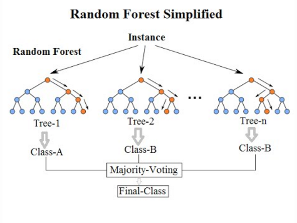
Random forests or random decision forests are an ensemble learning method for classification, regression and other tasks that operates by constructing a multitude of decision trees at training time and outputting the value that is the mode of the classes (classification) or mean/average prediction (regression) of the individual trees.
In simpler terms, the random forest algorithm creates multiple decision trees based on varying attributes and biases, and then predicts the output for each tree, and aggregates this prediction into one final output by some technique like majority count or average/etc.

Visual Representation of a Random Forest learning model. Credits: Random Forest Wikipedia
The main idea behind Random Forest arise from a method called ensemble learning method.
Ensemble learning is the method of solving a problem by building multiple ML models and combining them. It is primarily used to improve the performance of classification, prediction, and function approximation models.
Forests are type of ensemble learning methods, where they act like, pulling together all of decision tree algorithm efforts. Taking the teamwork of many trees thus improving the performance of a single random decision tree.
Random decision forests correct for decision trees’ habit of overfitting to their training set.
Now lets look at an example of prediction by the random forest model using the randomForest() function present in the randomForest library package. For more information about the randomForest() function and its attributes visit randomforest()
Thus following the 4 step method of prediction for predicting a numerical attribute “Earnings” using the randomForest() function.
We can see,
- the summary of the output randomForest model with details of:
- Formula used.
- Type of random forest
- Number of trees created in the forest
- Number of variables used at each split.
- And some performance parameter.
- The mean squared error of the predicted values using training sub-dataset.
- The mean squared error of the predicted values using the testing sub-dataset.
Note: Since a random forest is an ensemble learning method, it will usually take a lot more time to train that its counterparts. Thus you can see a significant waiting/execution time while running the above code and acquiring answer.
8.3 SVM
Support-Vector Machines (SVMs, also support-vector networks) are supervised learning models with associated learning algorithms that analyze data for classification(mostly) and regression(also works in some cases) analysis.
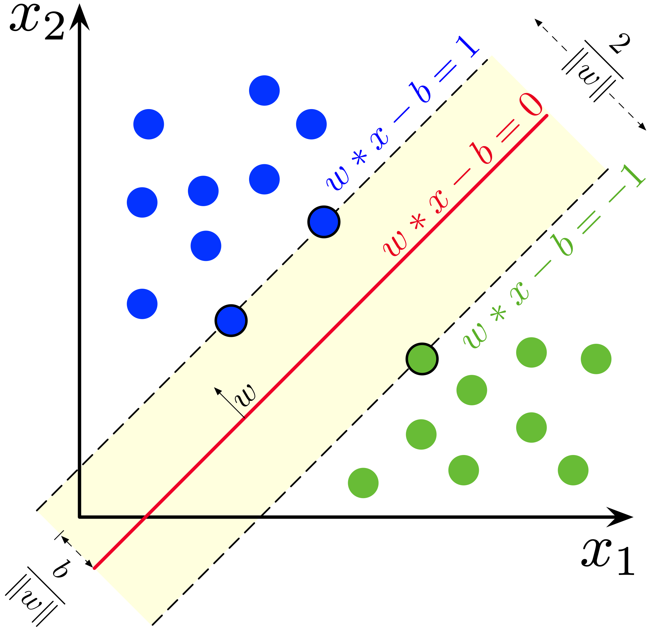
The goal of the SVM is to find a hyperplane in an N-dimensional space (where N corresponds with the number of features) that distinctly classifies/regresses the data points. The accuracy of the results directly correlates with the hyperplane that we choose. We should find a plane that has the maximum distance between data points of both classes.
Intuitively, a good separation is achieved by the hyperplane that has the largest distance to the nearest training-data point of any class (so-called functional margin), since in general the larger the margin, the lower the generalization error of the classifier.

Support Vector Machine Linear classification hyperplane(line) example. Credits: Support Vector Machines Wikipedia
Note that the dimension of the hyperplane depends on the number of features. If the number of input features is two, then the hyperplane is just a line. If the number of input features is three, then the hyperplane becomes a two-dimensional plane. It becomes difficult to draw on a graph a model when the number of features exceeds three.
In addition to performing linear classification, SVMs can efficiently perform a non-linear classification using what is called the kernel trick, implicitly mapping their inputs into high-dimensional feature spaces.

Example of the kernal trick for non-linear classifier. Credits: Support Vector Machines Wikipedia
Why is this called a support vector machine? Support vectors are data points closest to the hyperplane. They directly influence the position and orientation of the hyperplane and minimizes the margin of the classifier. Deleting the support vectors will change the position of the hyperplane. These points thus help to build our SVM model.
SVM is great because it gives quite accurate results with minimum computation power.
Lets look at the example of Support vector machine algorithm in use for predicting the Earnings attribute of the Earnings dataset.
We will use the svm() function from the e1071 package. For more information about this function and its attributes visit svm()
Thus following the 4 step model for prediction and using the “svm()” function as the model function.
We can see,
- the summary of the output svm model with details of:
- Formula used.
- Type of SVM model
- The SVM Kernel Used
- And some performance parameter.
- Also, the Number of Support Vectors.
- The mean squared error of the predicted values using training sub-dataset.
- The mean squared error of the predicted values using the testing sub-dataset.
8.4 Neural Network.
An Artificial Neural Network (ANN), usually simply called neural network(NN) is based on a collection of connected units or nodes called artificial neurons, which loosely model the neurons in a biological brain. Each connection, like the synapses in a biological brain, can transmit a signal to other neurons.
Thus in other words, a neural network is a sequence of neurons connected by synapses, which reminds of the structure of the human brain. However, the human brain is even more complex, and a NN is just a model that mimics a human brain.
An artificial neuron that receives a signal then processes it and can signal neurons connected to it. The “signal” at a connection is a real number, and the output of each neuron is computed by some non-linear function of the sum of its inputs. The connections are called edges.
Neurons and edges typically have a weight that adjusts as learning proceeds. The weight increases or decreases the strength of the signal at a connection. Neurons may have a threshold such that a signal is sent only if the aggregate signal crosses that threshold.
Typically, neurons are aggregated into layers. Different layers may perform different transformations on their inputs.
Signals travel from the first layer (the input layer), to the last layer (the output layer), possibly after traversing the layers multiple times.

A visual representation of typical neural network with various nodes and edges along with layers. Credits: Artificial Neural Network Wikipedia
What is great about neural networks is that they can be used for basically any task from spam filtering to computer vision. However, they are normally applied for machine translation, anomaly detection and risk management, speech recognition and language generation, face recognition, and more.
To accommodate such a wide variety of application, neural nets are transformed and models in various different ways. To find multiple types of neural networks please visit Neural Network Zoo
Now lets try to implement a neural network learning model for the Earnings prediction problem of Earnings dataset.
To do this we will use the 4 step method of prediction and use the nnet() function from the “nnet” package as the model_function.
Let look at the nnet() function and its parameters.
nnet(formula,data,size,linout,...)- formula and data are the same as mentions in Step 1 of section 8.1.
- size: denotes the number of units in the hidden layer.
- linout: Assign TRUE is predicting numerical value. Default is FALSE, for predicting categorical value.
- rang: set the initial random weights on each edge.
- maxit: maximum number of iterations.
- decay: weight decay parameter. Can also be understood as learning rate.
- Note: The nnet() function can only create a single hidden layer neural network model. To create more complex models please use different packages like neuralnet or h2o, deepnet, etc
Now lets use the nnet() function for predction.
NOTE: If you see a very high value of MSE after running the above code, please re-run it. Usually you will find the MSE to be better than all the models we have studied uptil now for the Earnings prediction problem.
We can see from the output,
- the summary of the output, neural network model, with details of:
- Number of weights in the complete neural network
- Initial Value and Final Value of the model weights along with iter value.
- Structure of the neural network in I-H-O format where the numbers, I is input, H is hidden and O is output nodes.
- Input node attributes.
- Note that the Majors column attribute are split into unique number of factors, thus creating new individual attributes.
- Output node attributes.
- Network Options.
- The mean squared error of the predicted values using training sub-dataset.
- The mean squared error of the predicted values using the testing sub-dataset.
After Comparing all these models, we can see that the MSE values for the 3 models are SVM > Random Forest > Neural Network. This suggest one trend that, to get as best result as possible, one must invest most time in choosing the right model,and use the model with cleaned dataset for training.
Eventually, since we use R language here, the code for model creation just boils down to few lines of code, 4 steps to be more accurate. But since we might find one model works better than other, we must choose the best fit model.
Also, we saw the trend of time required for training of the models studied above was SVM > RandomForest > Neural Net. This also suggest a proportional relationship with the time required for a particular model to train and in turn producing the best possible results.
Although one can say that, we can just use Neural Networks all the time, well this statement is true to some extent, but depending on the resources, the complexity of the data, and the complexity of the model itself, one needs to make some trade-offs. One should not try to throw a ball just few meters with a cannon, using mere hands will do the job. In essence, do not try to overuse the neural net model for the sake of adding 2 mumbers, simple addition will suffice. Studying these tradeoffs and more models in depth though is out of this course scope.
EOC